Algèbre linéaire
Python works with packages. A large number of packages can be dowloaded all together in the Anaconda environment. Start downloading here (version >3) https://www.anaconda.com/download/ Anaconda comes with
- Spyder, a GUI for python
- Jupyter Notebook, how to create great documents
Enjoy!
Bee careful :
- Python is sensible to spaces in the beginning of lines,
- Python is sensible to number type : $3$ and $3.$ are totally different: integer and float types.
import warnings
warnings.filterwarnings('ignore')
Back to basic instructions
Create a list filled with zeros
also_empty_list = []
zeros_list = [0] * 5
print(zeros_list)
Create empty list and fill it with elements : $append$
empty_list = list()
empty_list.append(1)
print(empty_list)
empty_list.append(2)
print(empty_list)
Return the length of a list : $len$
print(len(empty_list))
. . . . . . . . . .
. . . . . . . . . .
. . . . . . . . . .
. . . . . . . . . .
Loops
N=7
for i in range(N):
    print("Loop %d over %d. It means %d%%, approximately %f%%." % (i,N,i/N*100,i/N*100))
Functions
Python functions are defined using the $def$ keyword, then the name of the function, then $:$. A line break and indented lines. The result is returned to the user with $return$.
def ma_premiere_fonction(arg_1,times=5):
    return arg_1*times

# The second argument is not essential because initialised..
print(ma_premiere_fonction("top "))

# But if given, taken into account
print(ma_premiere_fonction("top ",24))
$if$ test
Let's create a function which tests the sign of the argument.
def sec_func(x):
    if x>0:
        return "positive"
    elif x<0:
        return "negative"
    else:
        return "zero"
print(sec_func(1.2))
print(sec_func(-31.2))
print(sec_func(1.2*0))
. . . . . . . . . .
. . . . . . . . . .
. . . . . . . . . .
. . . . . . . . . .
Matrices and vectors
import numpy as np
Let us begin with matrices $A$ and $B$ and vector $v$
$A=\begin{pmatrix} 2 & 3 & 1 \\ 0.5 & 2 & -1 \\ -1 & 5 & -7 \end{pmatrix},\quad B=\begin{pmatrix} 4 & 0 & 2 \end{pmatrix},\quad v=\begin{pmatrix} 5 \\ 3 \\ 2 \end{pmatrix}$
How to create those two objects ?
To create a matrix $A$
A=np.array([[2,3,1],
            [0.5,2,-1],
            [-1,5,-7]])
print(A)
To create a row matrix $B$...
B=np.array([[4,0,2]])
print(B)
...which is different from
B_vec=np.array([4,0,2])
print(B_vec)
v=np.array([[5],
            [3],
            [2]])
print(v)
Get dimensions
print(A.shape)
print(B.shape)
print(B_vec.shape) # Warning : returns uni-dimensional array
print(v.shape)
Basic matrix creations
a_0 = np.zeros((3,3))
print(a_0)
a_1 = np.ones((3,3))
print(a_1)
a_4 = np.full((3,3),4)
print(a_4)
a_id = np.eye(3)
print(a_id)
a_rd = np.random.random((3,3))
print(a_rd)
Concatenate vectors and matrices
mega_mat_1 = np.hstack([A,v,a_rd])
print(mega_mat_1)
mega_mat_2 = np.vstack([a_1,a_4])
print(mega_mat_2)
Extract array elements
$[,]$ permit to select particular elements. First coordinate for rows and second coordinate for columns.
print(A)
Extract $2$ to last columns and $1^{st}$ to $2^{nd}$ rows
A_1 = A[:2, 1:3]
print(A_1)
Extract All rows of $2^{nd}$ column
# Warning : returns uni-dimensional array
A_2_uni = A[:, 1]
print("BAD SOLUTION")
print(A_2_uni)
print(A_2_uni.shape)

A_2_bi = A[:, 1:2]
print("GOOD SOLUTION")
print(A_2_bi)
print(A_2_bi.shape)
Tests on elements
Look for larger than $2$ elements in $A$. To get the matrix with test results:
bool_id_A = (A>2)
print(bool_id_A)
To get the corresponding values:
print(A[A>2])
. . . . . . . . . .
. . . . . . . . . .
. . . . . . . . . .
Basic operations
x = np.array([[1,2],[3,4]])
y = np.array([[5,6],[7,8]])
Transpose
print(x.T)
Rank
np.linalg.matrix_rank(x)
Trace
np.trace(x)
Addition
print(x+3*y)
Matrix-product, also called dot-product
print(np.multiply(x, y))
Element-wise product
print(np.dot(x, y))
. . . . . . . . . .
. . . . . . . . . .
. . . . . . . . . .
Advanced operations
A=np.array([[1,0.1,0.7],
            [0.02,2,-0.2],
            [0.5,0.001,10]])
Determinant
print(np.linalg.det(A))
Inverse
print(np.linalg.inv(A))
. . . . . . . . . .
. . . . . . . . . .
Pour résoudre le problème, ayant $x$ pour inconnue, $Ax=b$
L'hypothèse forte est que $A$ soit inversible. On a vu dans le cours que le problème $Ax=b$, sous l'hypothèse précédente et où $b$ est un vecteur colonne a pour solution $$x=A^{-1}b,$$ Cce qui se traduit en python
A=np.array([[1,0.1,0.7],
            [0.02,2,-0.2],
            [0.5,0.001,10]])

b=np.array([[2],[5],[-8]])

print(np.linalg.solve(A,b))
a=1/2
A=np.array([[0,0,1,0],[0,0,0,1],[-a,a,0,0],[a,-a,0,0]])
np.round(np.linalg.eig(A)[0],7)**2
. . . . . . . . . .
About eigen-spaces /// A propos de la diagonalisation
How to get the "valeurs propres"
valeurs_propres = np.linalg.eigvals(A)
How to get the "vecteurs propres"
On va le faire en français, np.linalg.eig est la fonction utilisée pour estimer la décomposition diagonale de $A$. Ainsi
- $D$ est un np.ndarray qui contient les valeurs propres de la matrice $A$
- $P$ est un np.ndarray qui contient les vecteurs propres de la matrice $A$ On se souvient que si $v$ est un vecteur propre associé à la valeur propre $\lambda$ pour $A$, alors $$Av=\lambda v.$$ On a alors, en notant $D$ la matrice diagonale issue de l'output de la focntion np.linalg.eig, $$D=P^{-1}AP,$$ comme renseigné plus bas
D,P = np.linalg.eig(A)
D_estimated = np.dot(np.linalg.inv(P),np.dot(A,P))
print(D_estimated)
. . . . . . . . . .
Application au problème de physique
On se souvient que l problème de physique qui nous occupait ressemblait à ça
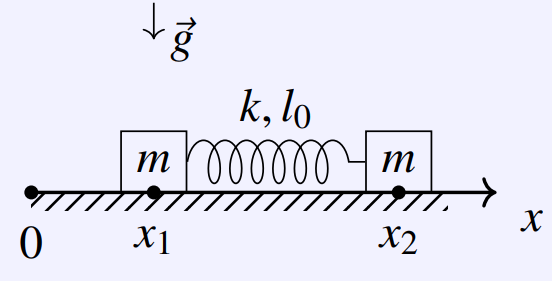
Que l'on a mis en équations pour se ramener au système suivant, où $\omega_0^2/2=k/l_0$ \begin{equation*} \left\{ \begin{array}{cl} x_1''&=\omega_0^2/2(x_2-x_1-l_0), \\ x_2''&=-\omega_0^2/2(x_2-x_1-l_0) \end{array} \right. \end{equation*}
Or, forts de ce que nous avons appris aujourd'hui, il est possible de réécrire le problème sous la forme diférentielle $$\ddot{X}=AX+b_0,$$ avec $A=\begin{pmatrix} -\omega_0^2/2 & \omega_0^2/2\\ \omega_0^2/2 & -\omega_0^2/2\\ \end{pmatrix}$, $X=\begin{pmatrix}x_1\\x_2\end{pmatrix}$ et $b_0=\omega_0^2l_0/2\begin{pmatrix}-1\\1\end{pmatrix}$.
Il ne reste plus qu'à résoudre en prenant les valeurs numériques proposées $\omega_0^2/2=1$ et $l_0=0.1$.
1) Donner la décomposition diagonale de $A$ : $(D,P)$.
omega_0_2_sur_2 = 1
l_0=0.1

A=omega_0_2_sur_2*np.array([[-1,1],[1,-1]])
b_0=omega_0_2_sur_2*l_0*np.array([[-1],[1]])
print(A)
D,P = np.linalg.eig(A)
print(np.round(D,4))
P_moins_1_b_0 = np.linalg.solve(P,b_0)
print(P_moins_1_b_0)
2) En déduire les paramètres des exponentielles solutions du problème.
En se souvenant que $\ddot{Y}=DY+P^{-1}b_0$ est un problème "simple" puisque $D$ est diagonale, il vient $$ \begin{array}{ll} \ddot{y_1}&=d_1y_1+(P^{-1}b_0)_1\\ \ddot{y_2}&=d_2y_2+(P^{-1}b_0)_2\\ \end{array}$$
d1,d2=np.round(D,2)
print(d1,d2)
Il vient donc $$Y(t)=\begin{pmatrix}y_1(t)\\y_2(t)\end{pmatrix}=\begin{pmatrix}C_1+E_1t\\C_2\cos(|d_2|t)+E_2\sin(|d_2|t)-(P^{-1}b_0)_2/d_2\end{pmatrix}.$$
4) En se souvenant que $X=PY$. Avec les conditions initiales $X(t=0)=(0,0.15)^T$ et $\dot{X}(t=0)=(0,0)^T$, tracer les évolutions temporelles de $x_1(t)$ et $x_2(t)$.
On sait que $X(t=0)=(0,0.15)^T$ et $X=PY$, alors $Y(t=0)=P^{-1}X(t=0)$
X_0 = np.array([[0],[0.15]])
Y_0=np.linalg.solve(P,X_0)
C1=Y_0[0]
C2=Y_0[1]+P_moins_1_b_0[1]/d2
print(C1)
print(C2)
De même que $\dot{X}(t=0)=(0,0)^T$ et $\dot{X}=P\dot{Y}$, alors $\dot{Y}(t=0)=P^{-1}\dot{X}(t=0)$. Mais tout est à $0$, donc:
E1,E2=0,0
Ainsi $$Y(t)=\begin{pmatrix}y_1(t)\\y_2(t)\end{pmatrix},$$
et alors $$X(t)=PY(t)=0.71\begin{pmatrix}y_1(t)-y_2(t)\\y_1(t)+y_2(t)\end{pmatrix},$$
import matplotlib.pyplot as plt

t = np.arange(0.0, 10.0, 0.1)

y_1 = C1
y_2 = C2*np.cos(np.abs(d2)*t)-P_moins_1_b_0[1]/d2

x_1 = 0.71*(y_1-y_2)
x_2 = 0.71*(y_1+y_2)

fig, ax = plt.subplots(1)
ax.plot(t,x_1, color='green',linewidth=2,label='$x_1(t)$')
ax.plot(t,x_2,color='red',linewidth=2,label='$x_2(t)$')
fig.suptitle('Déplacement versus temps', fontsize=20)
plt.xlabel('temps', fontsize=18)
plt.ylabel('Déplacement', fontsize=16)
handles, labels = ax.get_legend_handles_labels()
plt.legend()
plt.show()
5) Avez-vous des commentaires ?
. . . . . . . . . .
. . . . . . . . . .